Imitation Learning: How well does it perform?
We share a recent paper that provides a taxonomic framework and theoretical performance bounds for IL algos, then dive into into the craft of proving such bounds.
By Surya Vengadesan
Imitation learning (IL) broadly encompasses any algorithm (e.g. BC) that attempts to learn a policy for an MDP given expert demonstrations. In this blog post, we will be discussing how one can distinguish this task into three subclasses of IL algorithms with some mathematical rigor. In particular, we will be describing ideas presented in this recent paper that provides a taxonomixal framework for imitation learning algorithms.
A key idea behind this paper is to define a metric that generalizes the goal of IL algorithms at large. Simply put, find a policy that minimizes the imitation gap J(πE)−J(π), between our learned policy π and an expert policy πE. In particular, we define J(⋅), what we call a moment, which is the expection over some function.
The goal is to then match the expert and learner moments, which the paper refers to as moment matching. In particular each type of IL algorithm can be defined by different types of moments being matched, such as reward or Q functions. Through this lens, IL can be viewed as applying optimization techniques to minimize the imitation gap.
The paper then goes onto clearly defining the three types of IL algorithms and provides each with theoretical guarantees, proof after proof. Specifically, the author delineates between (1) matching rewards with access to the environment (2) matching q-values with access to the environment (3) matching q-values without access to the environment.
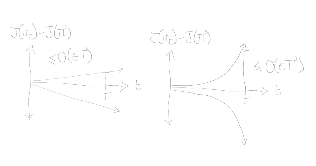
Now, we’ll attempt to deconstruct proofs from the paper on whether an algorithm’s imitation gap grows linearly or quadratically in time.
In particular, we will cover the paper’s first lemma which proves a linear upper bound on the imitation gap for type (1) algorithms that moment match reward functions like GAIL or SQIL. In the process, we will breakdown this craft of proving algorithmic bounds, then welcome the reader to decode the remaining proofs.
Lemma 1: Reward Upper Bound: If Fr spans F, then for all MDPs, πE and π←Ψ{ϵ}
That sounds like a handful; now, let’s break this down.
The author precedes this lemma with general framework that formalizes the goal of imitation learning algorithms. We should look at imitation learning as a two-player game. We define the payoff function of this game with U1 as follows:
Above, see the difference between two moments, the first moment over the sum of rewards till a time horizon T while following policy π, and the second moment over the sum of rewards till the same time horizon but following the expert policy πE. Therefore, given some expert policy πE, the game is to choose a policy π that best matches the moment of the expert, while being robust to all possible MDP reward functions f.
The paper defines Player 1 as the IL algorithm that attempts to select some policy π from the set of all possible policies
and whose goal is to minimize the imitation gap U1. Player 2 is a discriminating reward function f selected from the set of all reward functions Fr={S x A→[−1,1]}, whose goal is to maximize the imitation gap U1.
The notion of an δ-approximate solution to this game is also introduced. Given a payoff Uj, a pair (f^,π^) is a δ-eq. solution if:
In addition, we define a function that magically solves this game for us, which we call the imitation game δ-oracle, Ψ{δ}(⋅), which takes in in a payoff function
and returns a (kδ)-approximate equilibrium solution (f^,π^) that satifies the condition above.
Using the tools built up, we can now prove lemma 1. First one needs to use the imitation gap, based on it’s definition in the paper:
Next, since the sup is always positive, we can multiply by it by two and the new sup will be greater than one above. In addition, by defintion of U1, you can see that term we are taking the supremum over is simply T multiplied by U1. Therefore, we have:
Finally, if we apply the δ-approx. equilibrium def, we can see that:
Where f^ and π^, the optimal values can be seen as the result of performing the minimax over the policy class Π:
which is equal to 0 since, the expert policy πE∈Π, so U1 (as further defined above) collapses to 0.
Finally, we have that
and if you multiply this inequality by 2T, and bring the δ term to the right, you get
This matches the ϵ definition from the Lemma 1, so we finally get
The other lemma then goes onto proving that the lowerboard is also linearly constrainted.
Lemma 2: There exists an MDP, πE, and π←Ψ{ϵ}(U1) such that
However, takes on different techniques to prove the statement, which requires an in-depth understanding of more definitions to creatively chain together multiple logical tricks. Together, lemma 1 and 2 show that for any IL algorithm that attempts to match reward moments, its imitation gap will grow linear in both the best and worst case scenarios.
The paper goes on to prove bounds for the other two taxonomical categories, introduces a mathematical concept on MDPs called “recoverability”, and proposes two new algorithms using the proven bounds, one of which is called Adversarial Reward-moment Imitation Learning that is claimed to perform with better guaranteed performance over SQIL and GAIL.
If this material sounds interesting, check out the further readings below to get a glimpse into the world of Imitation Learning and how researchers today are incorporating rigor into the field in creative ways.
Also check out this youtube playlist created by Swamy et al. which gives an excellent overview of the work discussed in this blog.


