
How Maximum Entropy makes Reinforcement Learning Robust
Does information theory have a role to play in reinforcement learning? Find out how adding entropy to the reinforcement learning formulation can help robots deal with unexpected obstacles and more.


By Ashwin Reddy
This post explains what Shannon entropy is and why adding it to the classic reinforcement learning (RL) formulation creates robust agents, ones that tolerate unexpected, even adversarial, changes.
I’m assuming you’re familiar with general ideas in reinforcement learning so we can focus on intuition for why agents with high entropy are robust, in particular to changes in reward or changes in dynamics.
A Brief Review of RL
Recall that reinforcement learning aims to solve decision-making problems in games where a reward function r(s,a) assigns numerical points to action aaa in state sss of the game. Broadly, the goal is to determine how to score the most points (we’ll make this statement more concrete later).
The agent’s decision-making strategy, also known as its policy, denoted π, can be deterministic or stochastic. When repeatedly confronted with the same situation, a deterministic policy will always choose the same option whereas a stochastic policy selects according to a probability distribution over options.
For a concrete example of a stochastic policy, think of rock-paper-scissors. You wouldn’t play a deterministic policy against an intelligent opponent, because then they, knowing which option beats yours, could always win. Instead, you would make each option equiprobable, minimizing the opponent’s ability to exploit your strategy.
In truth, a deterministic policy is a stochastic policy; it takes a single action with probability 1. Thus, RL formalism typically takes the policy as a distribution over actions given the state, π(a|s ).
Since the policy is randomized, the total reward over the course of an episode of TTT steps is a random variable. To collapse this into a scalar objective, we take the expected value. The ideal policy maximizes this objective.
Enter Entropy
We’ll now introduce the second key ingredient.
In 1948, Claude Shannon, father of information theory, introduced the idea of entropy, a measurement of information for random variables, in his seminal paper “A Mathematical Theory of Communication.”
For Shannon, an event’s information content relates to how surprising it is. Information inversely correlates with probability of occurence since highly likely events are expected to happen anyway.
Say you’re playing Hangman. If you guess “e” and the word has an “e,” you didn’t discover much; “e” is the most frequent character in the English language. However, if you find that a “z” is in the word, that event provides lots of information since that drastically narrows the set of words under consideration.
Shannon’s desiderata for entropy also includes the following: supposing p1 and p2 are probabilities for independent events, the information I received from seeing both events is the information of seeing each event added together.
See if you can deduce why these criteria imply that the information of an event with probability p can be suitably defined as
The Shannon entropy H is compactly defined as the expected information content of a random variable X:
For simplicity, I supress details about differential entropy, which defines entropy for continuous random variables. For our purposes, the equation above applies to any random variable.
Entropy Intuition
A Bernoulli coin flip serves as a prototypical example for understanding entropy. Given X∼Bernoulli(p),
Let’s look at a plot. Entropy is measured in bits when the logarithm in I(p) has base 2.
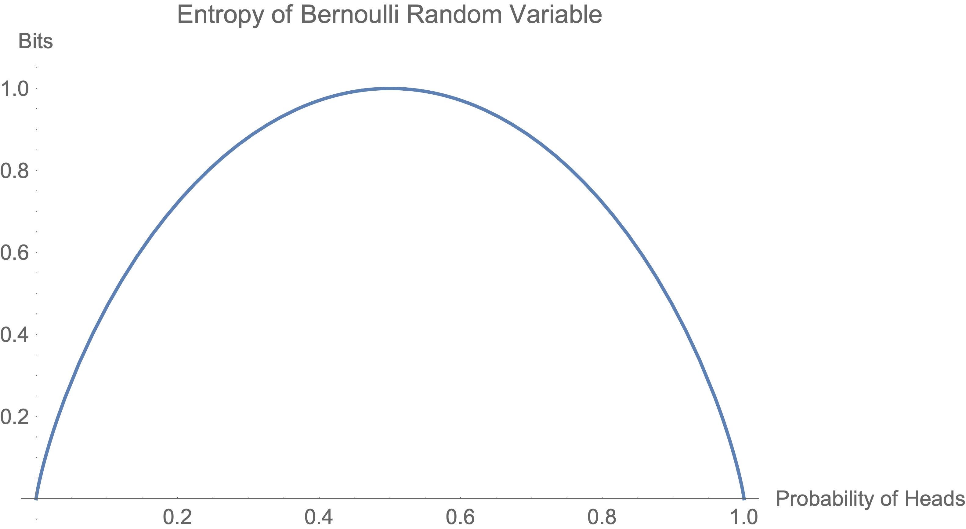
An equal chance of heads or tails maximizes entropy. However, as the probability of heads or tails becomes more and more certain (reaching 0 or 1), entropy decreases — we’re less surprised about the outcome.
Extending this logic, we see the uniform distribution has the highest entropy over all discrete random variables. Since no one option is more likely to show up, the outcomes give maximal surprise.
Maximum entropy distributions often play an important role in applications with uncertainty. For another example, let’s say you know a distribution has variance given by some constant σ2. Of all continuous distributions with variance σ2, the appropriate Gaussian distribution will have the highest entropy.
In rough terms, the uniform distribution and the Gaussian distribution, which maximize entropy subject to some constraints, minimize the amount of prior information they assume because they allow for the most surprise. As a result, qualitatively, higher entropy distributions tend to have a larger support (i.e. larger set of points with non-zero probability).
Concretely, if someone asked you to guess the probability of a heads for a possibly biased coin flip, it would make more sense to guess 50% rather than 100% or 0%. Or, if you had to guess what a random number generator will spit out, it would not be wise to bet it all on a single number.
MaxEnt RL
If we admit stochastic policies, reinforcement learning becomes a great application area for information theoretic concepts.
To that end, let’s think about how the entropy of an agent’s policy influences its actions. Entropy creates surprisal, so an agent with high entropy will actually have multiple strategies at its disposal simply by nature of policy’s randomness. In addition, we could interpret a maximum entropy policy distribution as making fewer assumptions about the world it’s in.
Thus, we hypothesize that encouraging entropy in our agents has beneficial properties. This formulation is exactly MaxEnt RL. We’ll include an entropy term as a bonus in the optimization.
What properties does this actually guarantee us?
If MaxEnt RL is the Answer, what is the Question?
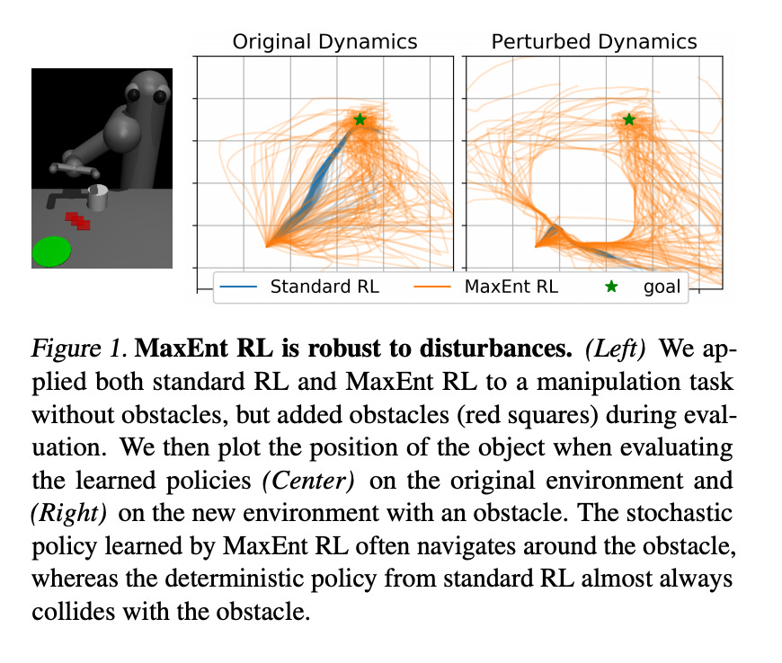
MaxEnt RL solves a variant of reinforcement learning called the robust reward problem. In the robust reward problem, the reward function is subject to change.
In other words, we have an adversarial player who gets to change how the agent is scored. Thus, we have a two-player zero-sum game; the agent needs to maximize its total reward in the worst case. The changes due to the adversarial player are higlighted in red.
where R is the set of reward functions the adversarial player can choose.
Proof
Let’s sketch the proof. First, we’ll look at cross-entropy, which tells us how much surprise to expect when we assume the events follow distribution q when they in fact come from a distribution p:
Naturally, the lowest cross-entropy comes when our assumption lines up with reality, i.e. p=q.
With some manipulation, the entropy term in the maximum entropy RL formulation can then be packaged into the reward function!
where
for any valid distribution q. In other words, MaxEnt RL ensures the highest reward under perturbations to the original reward function r(s,a).
Example
Let’s take the example from the paper to understand what’s at play here. Imagine a simple 2-armed bandit with reward
The robust set is given by adding in the perturbation from arbitrary distribution qqq.
We can then plot the robust set and see the associated rewards.

Robustness to Dynamics
We’ve now seen how MaxEnt RL is robust to variations in the reward. This insight actually enables us to make another claim about robustness: MaxEnt RL is also robust to changes in dynamics!
We won’t go into the proof (if you’re interested, that is covered in this blog post), but the high level idea is to convert variations in dynamics to variations in the reward.
Conclusion
We’ve built up some intuitive understanding of what entropy is and how it connects to RL agents. This connection combines rich insights from probability, information theory, and artificial intelligence. In particular, we can use these insights to encourage robustness to both rewards and dynamics in our agents. Robustness properties and guarantees may be useful for applications like robotics, where sensor information can be noisy and reward functions are not easy to write down. If you find these ideas interesting, I invite you to read the relevant papers!
Read More
Image References
 | A guest post by
|