
Neural Image Compression

By Selina Kim and Max Smolin
Even though computers have been rapidly getting better, the tasks we run on computers have also been getting harder and harder. Recently, an ever-growing share of the world’s computers works with Big Data, a marketing term roughly meaning “a lot more data than you think.” This means that computer storage efficiency, despite all the advances in the field, still requires incredible ingenuity.
Data compression is a large part of the problem of storage efficiency. It is basically a way to trade computational resources for the decrease in the sheer quantity of data stored. Many general algorithms that can be applied to any data whatsoever are known for this task, but specialized approaches allow for incredible efficiency for specific types of data.
In this article, we describe the ways of compressing image data in particular–starting from the traditional algorithmic approaches and building towards fancy new developments in the field of machine learning.
Before we spend time learning “how?”, however, we should answer the “why?”
Table of Contents
Motivation for Image Compression
The primary reason for studying the compression of image data is that there is a lot of it. The internet is full of pictures, from low-resolution user avatars all the way through 8K resolution computer desktop wallpapers. Each of these pictures takes up an immense amount of space (see the quantitative estimate below). In addition to that, images have to be sent over the internet in huge batches (think of an Instagram feed or a Facebook page full of vacation pics). Images also have to get to users really quickly since people typically refuse to wait for more than a second for a web page to load. Finally, video files are basically made up of thousands of images that have to be sent over the web in real-time, and image compression can help with that (although this task is so demanding that algorithms usually have to be adapted to exploit the time-wise properties of video).
All this makes for a pretty compelling reason to compress images, but not for why image compression deserves to be its own field. To demonstrate that, we note once again that domain-specific compression performs a lot better than generic compression, and also that images are actually highly resistant to artifacts. For example, humans are really bad at determining colors (except in relation to each other), so small errors in the color content of the image are likely to go unnoticed. People are also really good at filtering out small amounts of noise from images, etc. This means that an algorithm that can imperfectly compress images has a very real chance of replacing traditional general-case techniques (this is exactly what we see in practice with e.g., JPEG).
Now, let’s do some napkin mathematics to estimate the size of a small (by modern standards) image file, to further drive home the point of image data demanding compression.
Ignoring metadata, the size of the contents (in bytes) can be computed as follows:
Here, width and height are the dimensions of the image in pixels, and RGB stands for the 3 numbers (known as “channels”) that each represent a component of the color data, specifically the red, green, and blue color values. These are numbers from 0-255 and are usually the most popular way of encoding the colors of an image.
Substituting 1920 for width and 1080 for height, we get the size of an image that forms one frame of a Full HD (the highest widely available YouTube resolution) video:
This is already a very large amount, given that most use cases call for multiple images, and that most internet users these days use mobile internet with potentially very low speeds.
For example, if we consider a website such as Facebook, which needs to display dozens of vacation images displayed on each user’s feed (images tend to be 4032x3024, around 5.88 times larger than before), we can make a conservative estimate of the time it would take to download the images needed to display a page. The total size needed to display 12 images is
Now we divide that by the average LTE download speed:
This might not seem like that long, but realistically this is a ridiculously long time for a single small webpage to load. Facebook would not have many users without image compression, and its requirements for image loading are much tamer in comparison to power-users like Instagram. Basically, image compression is very often simply a business necessity.
Overview of Image Compression
Before going into the bells and whistles of convolutional neural networks—how does image compression work in general?
Images online are usually in PNG or JPEG format. In image compression, we can either conserve all information from an image with a lossless algorithm such as PNG, or we can lose some information about the image with a lossy algorithm such as JPEG. Luckily, most of the information we lose tends to be information that the human eye can’t detect. By losing some information, lossy compression algorithms can achieve a better compression ratio. Most neural image compression approaches focus on improving image compression for specific tasks. In this article, we will go over a lossy compressive autoencoder approach.
Entropy Encoding
Before we go over compressive autoencoders, let’s go over a non-neural image compression algorithm. If you are already familiar with entropy encoding, feel free to skip this section.
Let’s examine PNG, a lossless compression algorithm based on Huffman coding. Huffman coding is an entropy encoding method: it depends on knowing the probability with which some characters (say, in an alphabet) will occur. If we look at the English language, for instance, we can see that some letters occur in greater frequencies than others. For example, we rarely encounter the letters “x” or “z” in practice (in fact, until this point, this entire paragraph didn’t contain “z” at all!).
Here’s a graph of English letter frequencies in natural text (image taken from Wikipedia) to illustrate:
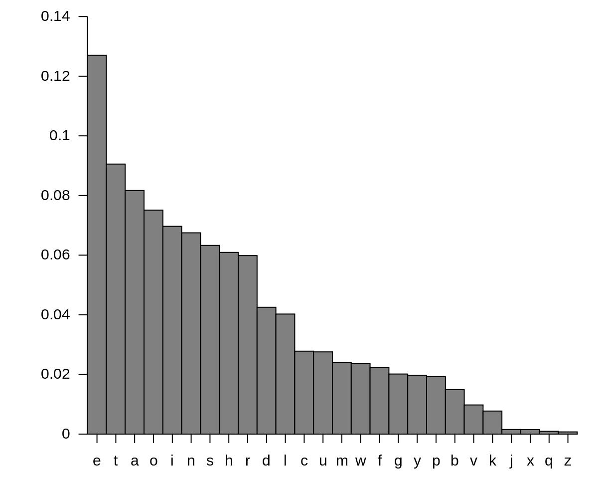
We can use Huffman coding to compress the number of bits needed to save some message in English. English has 26 letters, so we would need around 5 bits to encode the entire alphabet with fixed-length encoding: for instance, “a” might be encoded as “10000” while “b” is encoded as “10111”. But since we know that the letter “e” occurs very frequently, we can instead encode “e” with two bits—say “01”. In particular, Huffman coding is the optimal prefix coding (a code where the prefixes of all resulting codes are unique). Since “e” is “01”, the first two bits of any other letters’ encoding can not be “01”— “a” cannot be encoded as “011” for instance (an example of a valid encoding is “001”).
We can specialize Huffman coding to generate the optimal code for a particular message. A message or, in our case, an image, can be encoded in some optimal format: for instance, there may be a lot of “e” ‘s in a text message or a lot of red areas in a certain image. In Huffman encoding, we can use a binary tree to generate the optimal code, based on the probability or the frequency of each possible character the image. The resulting tree can be used to both decode and encode data.
Finding the probability of each possible character is not always easy: for example, PNG either goes through the entire image in order to generate a unique optimal binary tree for the image or uses pre-generated binary trees.
And since images are so complex, there are many ways to represent an image using entropy encoding: by pixels, bits or bytes, or using (as we will see later) the latent space representation of an image. PNG, in particular, chooses to compress images based on similar blocks of data in an image: rather than finding a probability distribution of individual bytes–PNG’s compression algorithm can find repetitive series of bytes in an image. Those series of bytes are then encoded via Huffman encoding.
Overview of Neural Image Compressors
Now that we’ve gone over how image compression generally works let’s consider how we can use machine learning to improve image compression.
Classical signal processing pipelines for image compression are designed by humans. This has the positive effect of bringing human intelligence and domain knowledge to the task but also has the negative effect of depending on human assumptions. Machine learning algorithms can (in theory) use the data to learn exactly what details are important and not important about images and exploit those properties to create a “perfect” compression algorithm.
As is always the case in machine learning, the first step to solving the problem is to define it with the best possible precision. This means specifying the following:
The type of the problem, in the case of neural image compression–self-supervised learning (target labels are created algorithmically from the input data, specifically where both the input and the target output are the image being compressed);
The loss function, which in the simplest case is a pixel-wise MSE–more on this later;
The model architecture.
There are two major approaches to neural image compression architectures. One is exploiting entropy encoding by creating a neural estimator of the probability of the image data. The other is compressive autoencoders. The first produces lossless compression, but as we know from our study of the classical methods, lossy image compression tends to be a better choice because small differences in images are inconsequential to humans. This is why we mainly concern ourselves with compressive autoencoders.
Compressive Auto-encoders
We will discuss the auto-encoder approach to neural image compression in-depth, using the 2017 paper by Lucas Theis, Wenzhe Shi, Andrew Cunningham, and Ferenc Huszár named Lossy Image Compression with Compressive Autoencoders as inspiration.
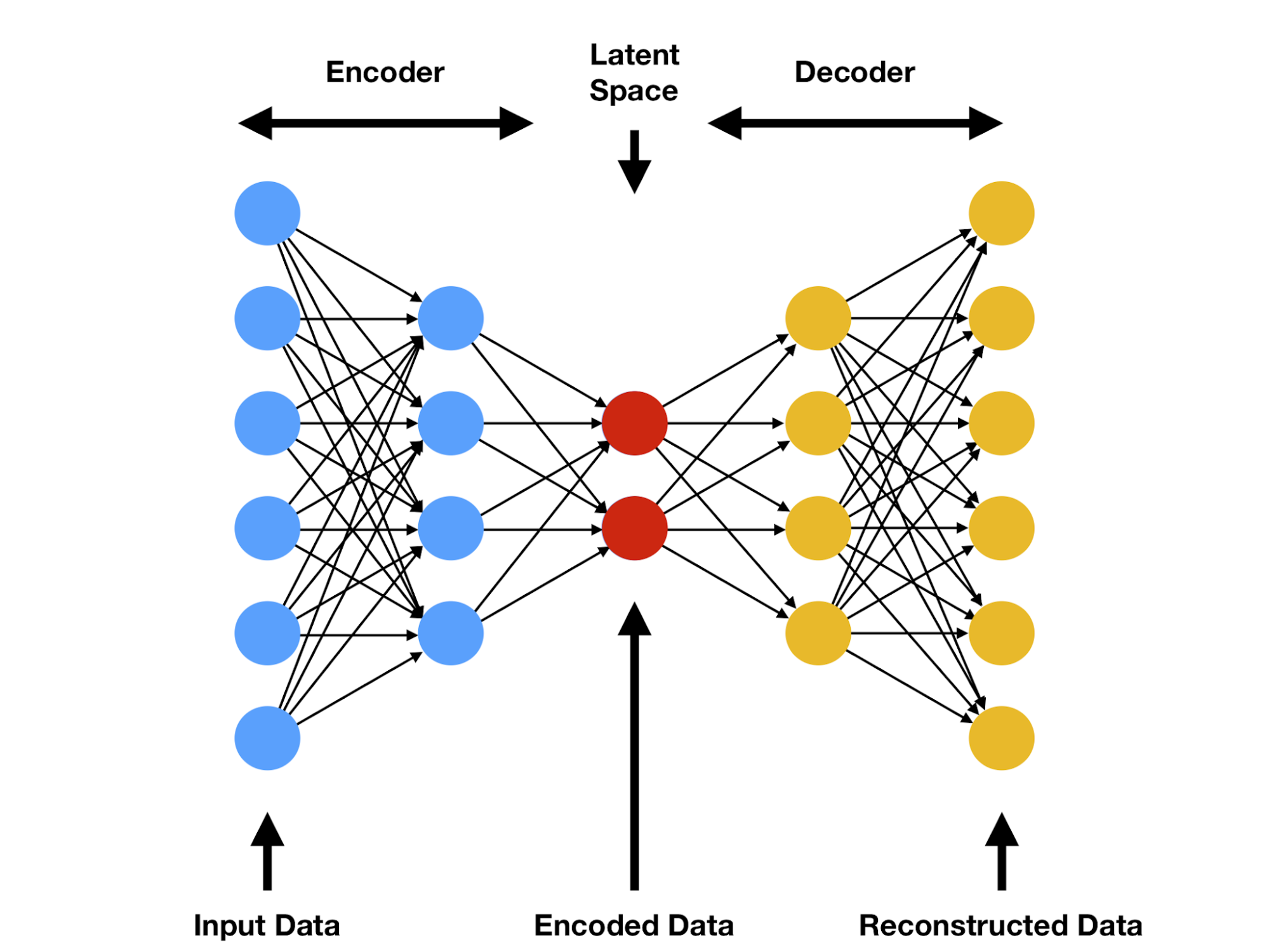
As a refresher, a short review of autoencoder models follows. An autoencoder model is named after its two primary functions–producing the input as its output (the “auto” prefix); and having an intermediate representation i.e., the “encoding,” formally called “latent space encoding.” This encoding is most often viewed as a “simpler” (in a way that varies model-to-model) representation of the input data.
This is usually achieved by introducing an informational bottleneck in the middle layers of the neural network, which prevents it from passing the input data to the output verbatim, thus requiring that a novel representation is learned.
A visual is provided below. This learned representation is, through gradient descent, expected to store the most “important” (according to the loss function) details of the input. In practice, latent space encodings are very useful for a wide variety of tasks. For example, taking the dot product between two latent space vectors often allows for a clever learned “similarity” network to be computed for the data that the autoencoder was trained on. The benefit of using autoencoder models is that the labels are trivially generated from the input data (target output = input data) and that the latent space can be arbitrarily shaped (given specific properties) using the loss function. We will discuss a specific autoencoder architecture in our study of the Compressive Autoencoder paper.
The main advantage of compressive auto-encoders, in addition to the high accuracy that they display in experiments (as shown in the paper by Theis et al.), is their similarity with other computer-vision tasks. For most designs, only a few changes are required to convert a neural network from classifying images to compressing images.
In particular, a neural network can be called a compressive auto-encoder if it fulfills the following criteria:
It must be an autoencoder, thus creating an intermediate (latent space) representation.
This intermediate implementation must be smaller in size (in bytes) than the original image, i.e., be a compressed version of it. This is somewhat different from the “bottleneck” that is typically present in non-compressive autoencoders. Normally, we assume that neural networks work with perfect mathematical numbers (infinite precision reals), but for the purposes of compression, we actually care about the exact bit counts. This means that the normal informational bottleneck would not actually work, since it is only intended to make it difficult to pass data verbatim, but does not provide any specific limits on the binary encoding size.
Now, we will go over the network proposed by Theis et al. and consider it under this framework:
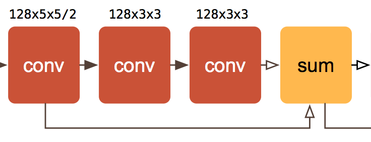
The first part of the network (i.e., the “encoder” required by our compressive autoencoder framework) is composed of two downsampling convolutions (downsampling is achieved by setting stride to 2), followed by three residual blocks (note that only two of these blocks are pictured below), and ending in another downsampling convolution.
The encoder is followed by an informational bottleneck in the form of a layer that rounds the floating-point intermediate representation to the nearest integer. This satisfies the second requirement of our framework.
The last part of the network (i.e., the “decoder” also required by our framework) is composed of a reversed version of the encoder. It is made of an upsampling layer that uses pixel shuffling (another name for subpixel convolutions, explained below), three residual layers, and two more upsampling layers using subpixel convolutions.
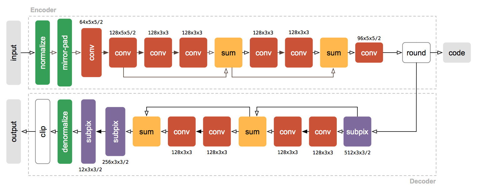
Figure 2: To reduce clutter, only two residual blocks of the encoder and the decoder are shown. Convolutions followed by leaky rectifications are indicated by solid arrows, while transparent arrows indicate absence of additional nonlinearities. The notation C × K × K refers to K × K convolutions with C filters. The number following the slash indicates stride in the case of convolutions, and upsampling factors in the case of sub-pixel convolutions.
There are a few important details that we will go over to further our understanding of the network:
Residual units play a very important role in modern neural image processing. They are the name of the convolution + sum + side connection union visible in the network diagram. The side connection is known as a “skip” or a “residual” connection These were introduced in the ResNet papers (Deep Residual Learning for Image Recognition and Identity Mappings in Deep Residual Networks) and are now considered a fundamental architectural building block. Adding residual connections allows for training deeper networks by propagating gradients more efficiently through the layers. This makes problems such as vanishing and exploding gradients incredibly uncommon since the gradient flows through the skip connections.
The rounding layer is non-differentiable by default, so the authors of the Compressive Auto-encoders paper replace its derivative with the identity to enable backpropagation.
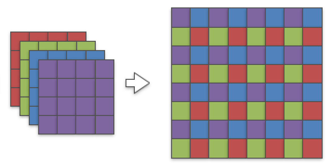
Subpixel convolutions are an equivalent reformulation of transposed convolutions (also sometimes called “deconvolutions”). In the latter, we consider the convolution as a matrix operation and transpose its matrix, which produces a new matrix that happens to upscale the image. Subpixel convolutions are implemented using a “pixel shuffle,” which redistributes channel data into spatial data. Here is a visual explanation:
You might have noticed that the auto-encoder model does not make use of entropy coding. This is indeed a great oversight in our simplified version of the model, but not the case in the original paper that uses this model instead:
At the top-right of the visualization above, there is now a new part, composed of a noise block and a GSM block. GSM here stands for Gaussian Scale Mixtures and represents a statistical method used in the paper to estimate the probability density function of the latent space. Using the probability of a given encoding (estimated by the GSM) the authors of the paper apply arithmetic coding to further decrease the size of the encoding. The loss function is also adjusted to not only take into account how dissimilar the reconstructed image is from the original but to also encourage the model to come up with predictable results that can be easily processed with arithmetic coding.
Image Loss Functions
There are different loss functions used in image processing. As expected, mean squared error makes an appearance since it’s easy to compute and a good general metric for errors in signals.
MSE is extremely useful under certain circumstances. For instance, it assumes that the spatial relationship of data samples does not matter. Every data sample is also considered to be equally important.
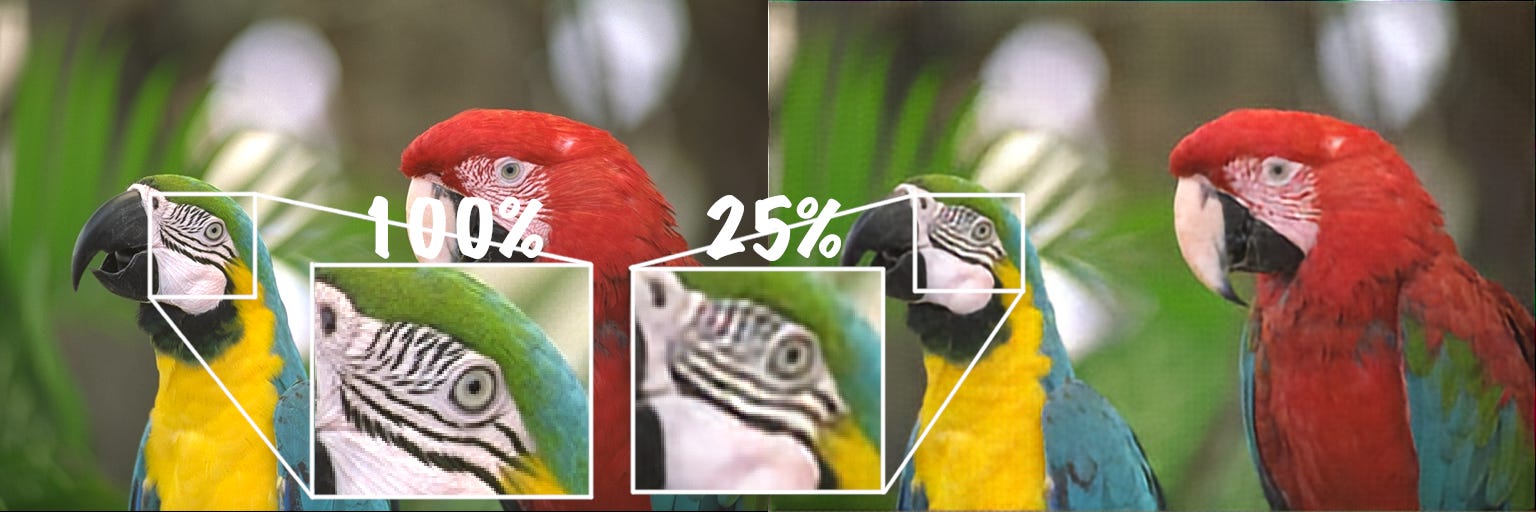
However, loss functions in problems concerning images are unique because the human visual system has certain biases—these biases help us view the world more clearly, but they make it difficult to accurately quantify image quality as perceived by humans. The human visual system is less sensitive to changes under certain circumstances: for instance, in places with high contrast or high luminescence, humans don’t perceive image distortions as much. So mean squared error, while computationally efficient, isn’t the most accurate method of determining image quality since it ignores the specifics of what people consider important in images.
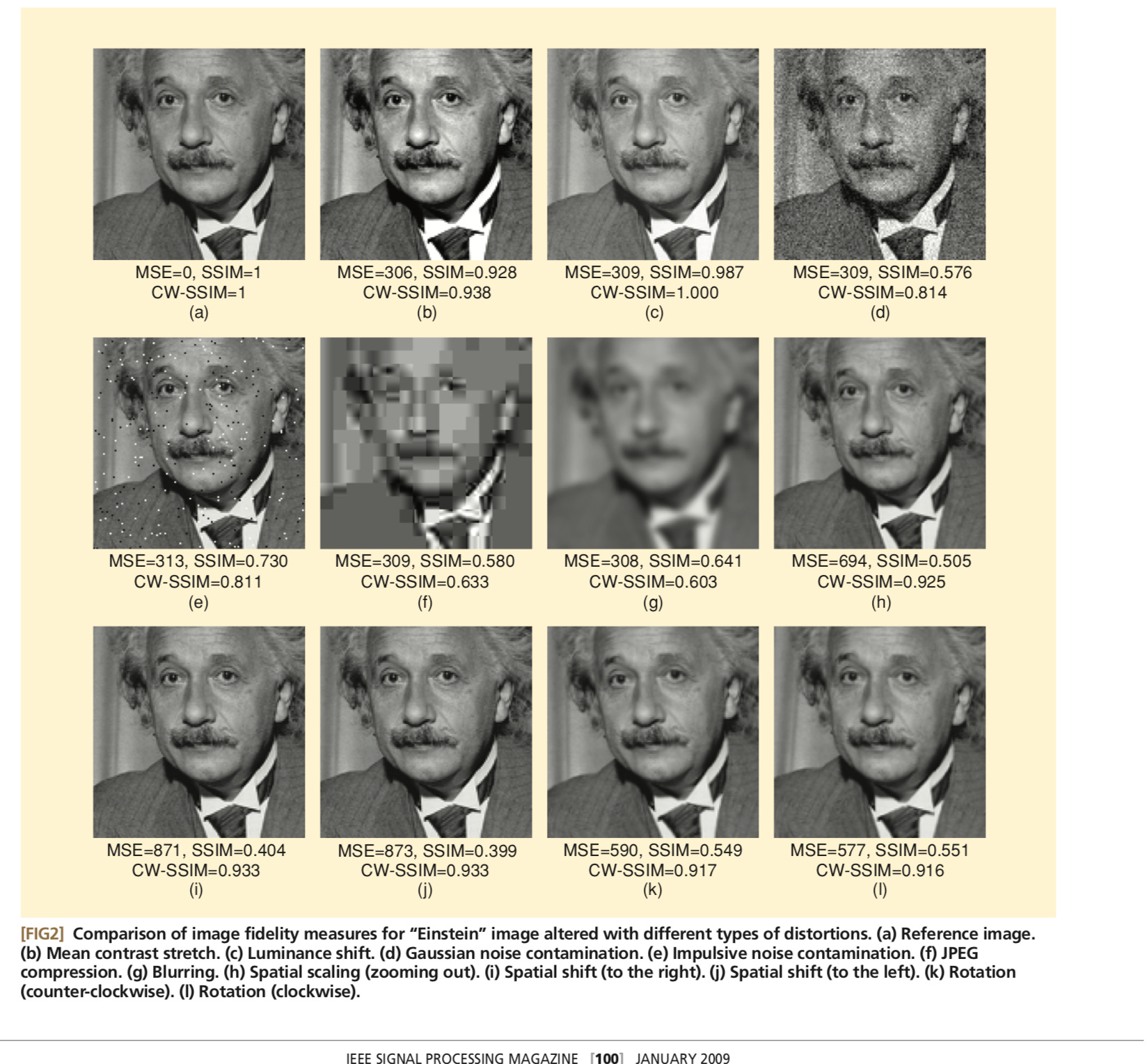
Imagine if we take an image A and outright replace a few bright-colored pixels with black pixels to make a new image B. To a human, the altered image B may look very similar to the original image A, but the MSE between the two images may be quite high. It’s possible to take A again and distort it to create another image C, such that B and C have the same MSE in comparison to the original image A. Only for image C, let’s say we blur the image. In this case, all the pixels are different but only by a very small amount. Most importantly, since the image is blurred (which people are very sensitive to), a human would perceive C to be very different from A, but the MSE of C and the MSE of B would be the same.
This is why an alternative loss function, called the Structural Similarity Index (or SSIM) is used—it’s a metric designed for quantifying image/video quality. However, since SSIM requires more calculations, it is less useful if there aren’t enough compute resources while training. SSIM compares the differences between images (e.g., an original and a compressed version) based on the following three factors: luminance, contrast, and structure. Two nnn-by-nnn windows xxx and yyy in an image are thus compared
where l(x,y), c(x,y), and s(x,y) are functions that compare the windows based on the aforementioned factors.
This is drastically more accurate in quantifying human perception of image quality. Consider the diagram below showing the SSIM and MSE of different images, from the article “Mean Squared Error: Love It or Leave It?” in the IEEE Signal Processing Magazine:
A number of more advanced variations of SSIM exist that are meant to improve the accuracy of the algorithm by considering the different parameters that can affect image quality, although SSIM considers most of the important biases (due to its focus on the human visual system). Multi-scale Structural Similarity Index (MS-SSIM), for instance, is an algorithm that calculates the SSIM of an altered image at different resolutions. This improves the resulting metric because the perceived quality of an image can drastically change based on the image scale (a viewer’s proximity to an image, the display resolution, etc.).
Finally, we would like to note that most modern papers on image processing provide measurements of Mean Squared Error, SSIM, and some flavor of SSIM. So really, the consensus on which metric is the best is to use all of them at once. Some papers even go as far as to have panels of people rate the results subjectively, showing that researchers are not really ready to put their trust in any of the aforementioned functions. The takeaway here is probably to use some variant of SSIM for training (at least in the later epochs to get rid of the idiosyncrasies of MSE), and to provide as many metrics as you can muster in your results.
Conclusion
We have discussed how image compression enables us to virtually send a ridiculous amount of images over the internet, which is crucial for social media and businesses based on social media. Discussing the more traditional approaches to image compression, we discovered that biasing our interpretation of image data to be more inline with human perception turns out to be beneficial. Since it is very difficult to model what humans think, we studied the application of the most advanced tool currently available for the task–neural networks. But what is the big picture here?
Since image data (and especially our ability to understand it) is incredibly important for things ranging from analyzing medical scans to searching through security footage, it is unlikely that images are going to become any less prominent in the future. This is why novel image compression techniques will probably continue to be developed. For instance, we may want to develop an image compression algorithm that effectively compresses medical scans of a patient for storage: this problem would have to take into consideration the properties of the specific problem (going beyond adjusting for human perception) and what sort of information should be preserved to be truly effective (it probably would not preserve the halo introduced around the organ by the scanner’s lamp). Machine learning, as we have hopefully demonstrated in this post, has been incredibly successful at creating systems that can devise and exploit such complicated insight into data, and will likely be the next big thing in image compression software.