
Neural ODEs

By Aidan Abdulali
In this post, we explore the deep connection between ordinary differential equations and residual networks, leading to a new deep learning component, the Neural ODE. We explain the math that unlocks the training of this component and illustrate some of the results. From a bird’s eye perspective, one of the exciting parts of the Neural ODEs architecture by Ricky T. Q. Chen, Yulia Rubanova, Jesse Bettencourt, and David Duvenaud is the connection to physics. ODEs are often used to describe the time derivatives of a physical situation, referred to as the dynamics. Knowing the dynamics allows us to model the change of an environment, like a physics simulation, unlocking the ability to take any starting condition and model how it will change. With Neural ODEs, we don’t define explicit ODEs to document the dynamics, but learn them via ML. This approach removes the issue of hand modeling hard to interpret data. Ignoring interpretability is an issue, but we can think of many situations in which it is more important to have a strong model of what will happen in the future than to oversimplify by modeling only the variables we know. NeuralODEs also lend themselves to modeling irregularly sampled time series data. The standard approach to working with this data is to create time buckets, leading to a plethora of problems like empty buckets and overlaps in a bucket. The NeuralODE approach also removes these issues, providing a more natural way to apply ML to irregular time series.
Table of Contents
Residual Networks
To explain and contextualize Neural ODEs, we first look at their progenitor: the residual network. In a vanilla neural network, the transformation of the hidden state through a network is
where f represents the network, ht is the hidden state at layer t (a vector), and θt are the weights at layer t (a matrix). The hidden state transformation within a residual network is similar and can be formalized as
The difference is we add the input to the layer to the output of the layer.
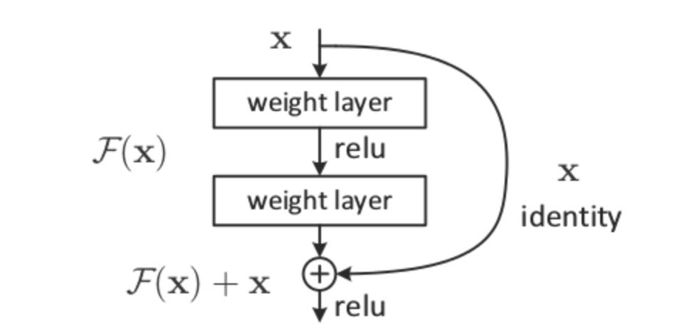
Why do residual layers help networks achieve higher accuracies and grow deeper? Firstly, skip connections help information flow through the network by sending the hidden state, ht, along with the transformation by the layer, f(ht), to layer t+1, preventing important information from being discarded by f. As each residual block starts out as an identity function with only the skip connection sending information through, depth can be incrementally introduced to the network via training fff after other weights in the network have stabilized. If the network achieves a high enough accuracy without salient weights in f, training can terminate without fff influencing the output, demonstrating the emergent property of variable layers.
Secondly, residual layers can be stacked, forming very deep networks. Introducing more layers and parameters allows a network to learn a more accurate representations of the data. But why can residual layers be stacked deeper than layers in a vanilla neural network? To answer this question, we recall the backpropagation algorithm. To calculate how the loss function depends on the weights in the network, ∂L/∂θ, we repeatedly apply the chain rule on our intermediate gradients, multiplying them along the way. These multiplications lead to vanishing or exploding gradients, which simply means that the gradient approaches 0 or infinity. Gradient descent relies on following the gradient to a decent minima of the loss function. A 0 gradient gives no path to follow and a massive gradient leads to overshooting the minima and huge instability.
As introduced above, the transformation
can represent variable layer depth, meaning a 34 layer ResNet can perform like a 5 layer network or a 30 layer network. Thus ResNets can learn their optimal depth, starting the training process with a few layers and adding more as weights converge, mitigating gradient problems. Thus the concept of a ResNet is more general than a vanilla NN, and the added depth and richness of information flow increase both training robustness and deployment accuracy.
However, ResNets still employ many layers of weights and biases requiring much time and data to train. On top of this, the backpropagation algorithm on such a deep network incurs a high memory cost to store intermediate values. ResNets are thus frustrating to train on moderate machines.
Differential Equations and Euler’s Method
The rich connection between ResNets and ODEs is best demonstrated by the equation
As stated above, this relationship represents the transformation of the hidden state during a single residual block, but as it is recursive, we can expand into the sequence below in which i is the input:
To connect the above relationship to ODEs, let’s refresh ourselves on differential equations. They relate an unknown function y to its derivatives. The solution to such an equation is a function which satisfies the relationship. Let’s look at a simple example: y′(x)=ky(x). This equation states “the first derivative of y is a constant multiple of y,” and the solutions are simply any functions that obey this property! For this example, functions of the form
obey this relationship. To solve for the constant A, we need an initial value for y. Let’s say y(0)=15. Solving
tells us A=15. This sort of problem, consisting of a differential equation and an initial value, is called an initial value problem.
Often times, differential equations are large, relate multiple derivatives, and are practically impossible to solve analytically, as done in the previous paragraph. Thankfully, for most applications analytic solutions are unnecessary. The value of the function y at time t is needed, but we don’t necessarily need the function expression itself. Even more convenient is the fact that we are given a starting value of y in an initial value problem, meaning we can calculate y′ at the start value with our DE.
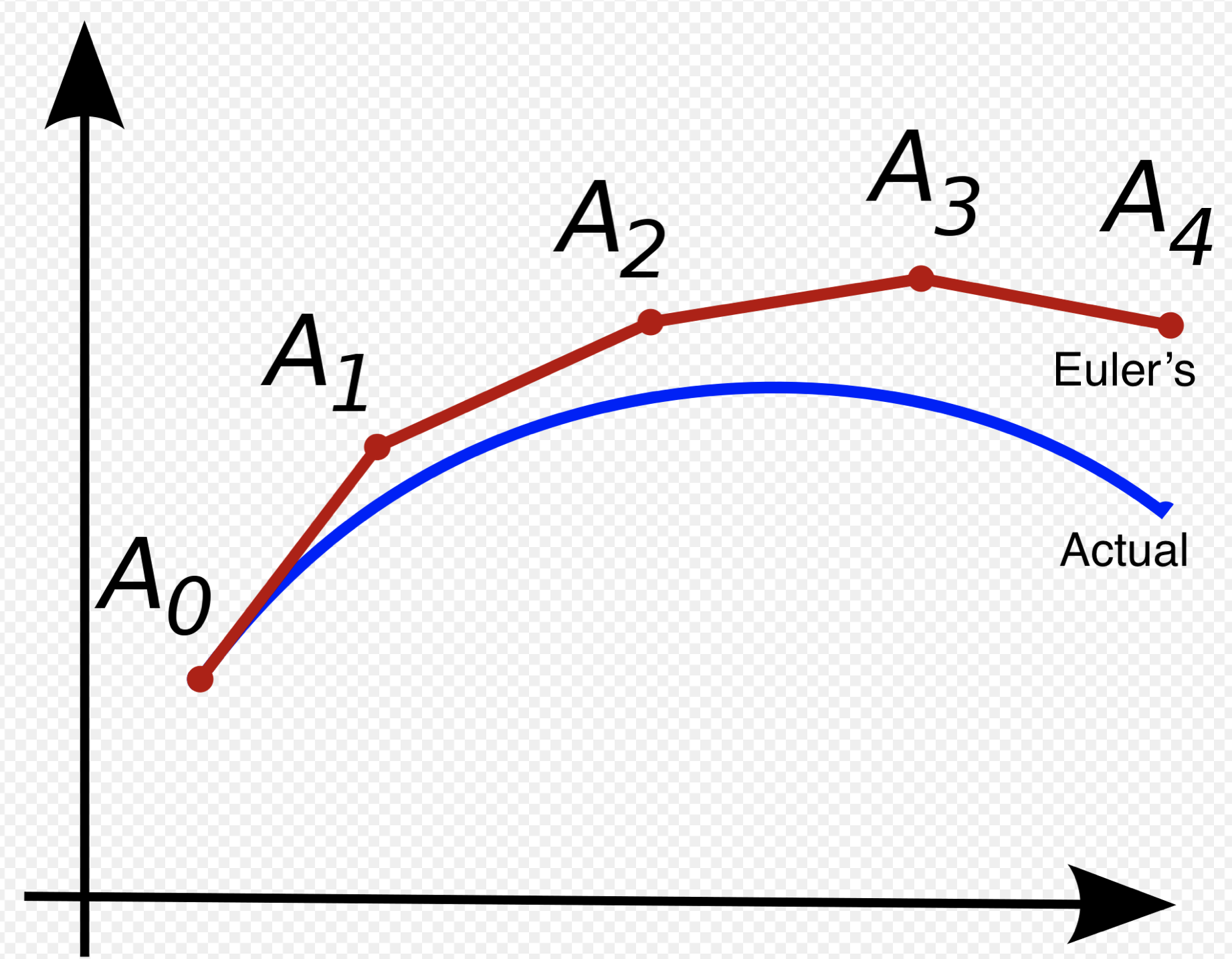
As seen above, we can start at the initial value of y and travel along the tangent line to y (slope given by the ODE) for a small horizontal distance of t, denoted as s (step size). Our value for y at t0 + s is y1=y0 + sy′(0). We can repeat this process until we reach the desired time value for our evaluation of y. The recursive process is shown below:
Hmmmm, doesn’t that look familiar! This numerical method for solving a differential equation relies upon the same recursive relationship as a ResNet. Let’s look at how Euler’s method correspond with a ResNet. In Euler’s we have the ODE relationship y′=f(y,t), stating that the derivative of y is a function of y and time. Next we have a starting point for y, y(0). How does a ResNet correspond? In a ResNet we also have a starting point, the hidden state at time 0, or the input to the network, h0. Instead of an ODE relationship, there are a series of layer transformations, f(θt), where t is the depth of the layer. These transformations are dependent on the specific parameters of the layer, θt. These layer transformations take in a hidden state f(θt, ht-1) and output
the hidden state to be passed on to the next layer, ht. This is analogous to Euler’s method with a step size of 1.
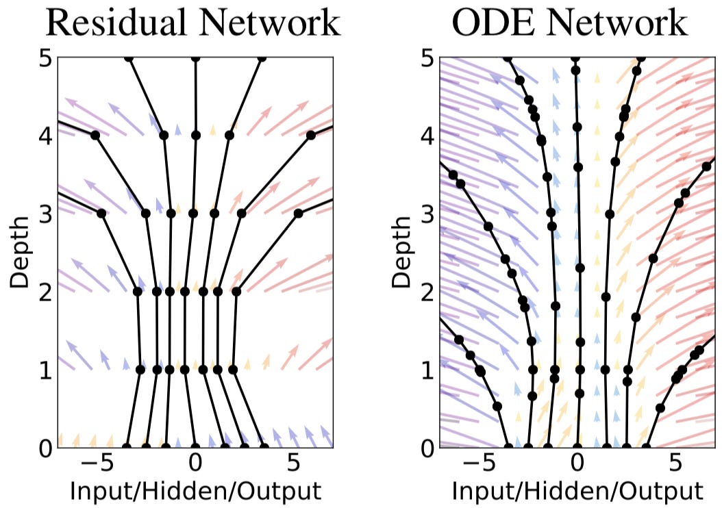
Even though the underlying function to be modeled is continuous, the neural network is only defined at natural numbers t, corresponding to a layer in the network. In the figure below, this is made clear on the left by the jagged connections modelling an underlying function. However, only at the black evaluation points (layers) is this function defined whereas on the right the transformation of the hidden state is smooth and may be evaluated at any point along the trajectory.
Differential equations are defined over a continuous space and do not make the same discretizations as a neural network, so we modify our network structure to capture this difference to create an ODENet
ResNet:
def f(z, t, 𝛳):
    return nnet(z, 𝛳_t)

def ResNet(z, 𝛳):
    for t in range(1, T):
        z = z + f(z, t, 𝛳)
    return z
ODENet:
def f(z, t, 𝛳):
    return nnet([z,t], 𝛳)

def ODENet(z, 𝛳):
    for t in range(1, T):
        z = z + f(z, t, 𝛳)
    return z
The primary differences between these two code blocks is that the ODENet has shared parameters across all layers. Without weights and biases which depend on time, the transformation in the ODENet is defined for all t, giving us a continuous expression for the derivative of the function we are approximating. Another difference is that, because of shared weights, there are fewer parameters in an ODENet than in an ordinary ResNet. For example, a ResNet getting ~0.4 test error on MNIST used 0.6 million parameters while an ODENet with the same accuracy used 0.2 million parameters!
In the ODENet structure, we propagate the hidden state forward in time using Euler’s method on the ODE defined by f(z,t,θ). However, we can expand to other ODE solvers to find better numerical solutions. With over 100 years of research in solving ODEs, there exist adaptive solvers which restrict error below predefined thresholds with intelligent trial and error. These methods modify the step size during execution to account for the size of the derivative. For example, in a ttt interval on the function where f(z,t,θ) is small or zero, few evaluations are needed as the trajectory of the hidden state is barely changing. But when the derivative f(z,t,θ) is of greater magnitude, it is necessary to have many evaluations within a small window of ttt to stay within a reasonable error threshold.
There are some interesting interpretations of the number of times ddd an adaptive solver has to evaluate the derivative. If d is high, it means the ODE learned by our model is very complex and the hidden state is undergoing a cumbersome transformation. Meanwhile if d is low, then the hidden state is changing smoothly without much complexity. Thus, the number of ODE evaluations an adaptive solver needs is correlated to the complexity of the model we are learning. In terms of evaluation time, the greater d is the more time an ODENet takes to run, and therefore the number of evaluations is a proxy for the depth of a network. In adaptive ODE solvers, a user can set the desired accuracy themselves, directly trading off accuracy with evaluation cost, a feature lacking in most architectures.
With adaptive ODE solver packages in most programming languages, solving the initial value problem can be abstracted: we allow a black box ODE solver with an error tolerance to determine the appropriate method and number of evaluation points. The pseudocode is shown below.
AdaptiveODENet:
def f(z, t, 𝛳):
    return nnet([z,t], 𝛳)

def ODENet(z, 𝛳):
    z = ODESolver(f, z, 0, t, 𝛳)
    return z
Training ODENets
Continuous depth ODENets are evaluated using black box ODE solvers, but first the parameters of the model must be optimized via gradient descent. To do this, we need to know ∂L/∂θ: how the loss function depends on the parameters in the ODENet. In deep learning, backpropagation is the workhorse for finding ∂L/∂θ, but this algorithm incurs a high memory costs to store the intermediate values of the network. On top of this, the sheer number of chain rule applications produces numerical error. Since an ODENet models a differential equation, these issues can be circumvented using sensitivity analysis methods developed for calculating gradients of a loss function with respect to the parameters of the system producing its input.
To get the gradient of the loss function with respect to the parameters of the network, we must first calculate how the loss depends on the hidden state of the network at time t: z(t). This intermediate step is standard in the backprop algorithm as well.
Knowing how z(t) changes with respect to time allows us to calculate the hidden state at any point. We can make this calculation because we have a starting value, the result of the network, and if we know the ODE which governs the hidden state we can solve an initial value problem backwards in time to get the hidden state for any ttt. This ODE is exactly what our ODENet defines! Thus dz(t)/dt is equal to our ODENet, symbolized by f(z(t),t,θ).
To help focus on what we want to achieve, we perform a substitution and define a vector which is the derivative of the loss with respect to the hidden state at a specific time t. We call this the adjoint state: a(t)=dL/dz(t). To clarify, we are now searching to define a(t) for all t to understand how the loss depends on the hidden state along its trajectory.
At the output of the network, this is easy to achieve as we can take the derivative of the loss function with respect to each component of the output vector and find a(toutput). To propagate further back in time, we wish to find a formula for da(t)/dt. This is more tricky, so let’s take a step back and examine the analogue of dL/dz(t) in the discrete case.
Recall that the chain rule for backprop:
We can try to convert this equation to the continuous case:
We have defined everything in the above equation except for z(t+ϵ), so a natural next step is to pin down this term. We know the derivative of z(t) is described by f(z(t),t,θ), so we can easily find the change in z(t) from t to t+ϵ by integrating f(z(t),t,θ) with respect to t over the interval:
By adding the starting point, z(t), to this integral, we find a full expression for our term:
For ease in the following derivations, we will call this term
Let’s plug all the terms we know into the continuous chain rule equation,
We recall that we previously defined dL/dz(t) as a(t), and we just found the expression Tϵ(z(t),t) for z(t+ϵ), so we are left with
What is left is to take the time derivative of
to arrive at our intermediary term da(t)/dt. This calculation is a bit tedious and only relies on basic calculus, so we omit it here. Refer to appendix B.1 or the Neural ODE paper if you would like to see it.
The conclusion is that
This equation unlocks the ability to calculate a(t) for any t. By taking the derivative of the loss function with respect to each component of the output vector, we get a(toutput) and can use this as our initial value in an initial value problem. The other component of course is da(t)/dt, which we just found. We can solve the initial value problem backwards in time, using the equation
allowing us to access how the loss function depends on the hidden state at any point in its trajectory.
The next and final portion of this calculation is to get gradients of the loss function with respect to the parameters of the network. The first set of important parameters are the weights and biases in the network, θ. Since a Neural ODE propagates a hidden state forward in time from t0 to tn, we also want derivatives with respect to these values. We will proceed similarly to the calculation of dL/dz(t), by defining an adjoint state. Instead of separating this calculation from the above one for a(t), we can augment the adjoint state to encompass the new variables, t and θ, which we would like to find the loss function’s dependence upon. We thus define the full dynamics of the system, which includes not only how the adjoint changes with respect to time but also how the parameters and time changes with respect to time:
The first partial derivative is equal to 1, as the time depends directly upon itself and the second partial derivative is equal to 0, as the parameters are constant throughout the network:
This equation describes how the variables of the system, z,θ,tz, change with respect to time. We have augmented our original adjoint state to include the time dependencies of the parameters and time. As we did before with a(t)=dL/dz(t), we can use the previous notation:
where az is our previously defined adjoint state, ∂L/∂z(t),
We would like to know the function faug( [z,θ,t] ) changes with respect to its input parameters, allowing us to understand the dependencies of the loss function across all t. The way to express this in multivariable calculus is with a Jacobian, which is the matrix of a function’s first order partial derivatives. The Jacobian of faug is
Previously, we defined the dynamics of the adjoint state as
We can substitute the corresponding parts for the augmented adjoint state, shown below:
We now have the augmented adjoint dynamics, and can integrate backwards in time to get the gradient of the loss function with respect to the parameters of the network, like we did before with the loss function with respect to the hidden state. The second term in daaug(t)/dt describes the dynamics of ∂L/∂θ(t), so we can integrate this over the whole hidden state trajectory to find
The value of ∂L/∂tn is given by a(tn)f(z(zn),tn,θ), since this is the evaluation at the output of the network and can readily be computed without integration.
The third term in daaug(t)/dt describes the dynamics of the ∂L/∂t, so we subtract the integral over the hidden state trajectory from the final value, ∂L/∂tn, to find ∂L/∂t0:
Neural ODEs for Supervised Learning
In the Neural ODE paper, the first example of the method functioning is on the MNIST dataset, one of the most common benchmarks for supervised learning. It contains ten classes of numerals, one for each digit as shown below.
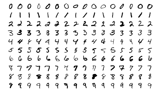
The task is to try to classify a given digit into one of the ten classes. To achieve this, the researchers used a residual network with a few downsampling layers, 6 residual blocks, and a final fully connected layer as a baseline. For the Neural ODE model, they use the same basic setup but replace the six residual layers with an ODE block, trained using the mathematics described in the above section. They also ran a test using the same Neural ODE setup but trained the network by directly backpropagating through the operations in the ODE solver. Along with these modern results they pulled an old classification technique from a paper by Yann LeCun called 1-Layer MLP. The results are very exciting:
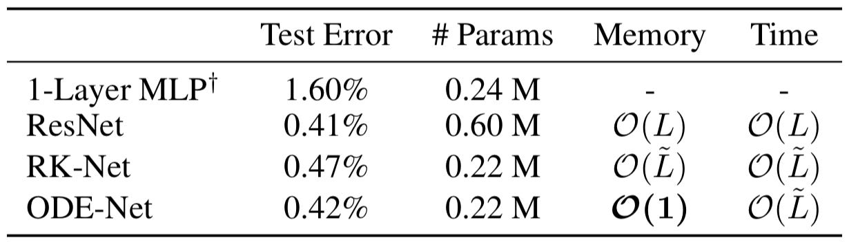
Disregarding the dated 1-Layer MLP, the test errors for the remaining three methods are quite similar, hovering between 0.5 and 0.4 percent. The big difference to notice is the parameters used by the ODE based methods, RK-Net and ODE-Net, versus the ResNet. The ResNet uses three times as many parameters yet achieves similar accuracy! This tells us that the ODE based methods are much more parameter efficient, taking less effort to train and execute yet achieving similar results. The next major difference is between the RK-Net and the ODE-Net. The RK-Net, backpropagating through operations as in a standard neural network training uses memory proportional to L, the number of operations in the ODESolver. This scales quickly with the complexity of the model. However, the ODE-Net, using the adjoint method, does away with such limiting memory costs and takes constant memory! This is amazing because the lower parameter cost and constant memory drastically increase the compute settings in which this method can be trained compared to other ML techniques. For mobile applications, there is potential to create smaller accurate networks using the Neural ODE architecture that can run on a smartphone or other space and compute restricted devices.
Limitations of Neural ODEs
Above, we demonstrate the power of Neural ODEs for modeling physics in simulation. The results are unsurprising because the language of physics is differential equations. The connection stems from the fact that the world is characterized by smooth transformations working on a plethora of initial conditions, like the continuous transformation of an initial value in a differential equation. Below, we see a graph of the object an ODE represents, a vector field, and the corresponding smoothness in the trajectory of points, or hidden states in the case of Neural ODEs, moving through it:
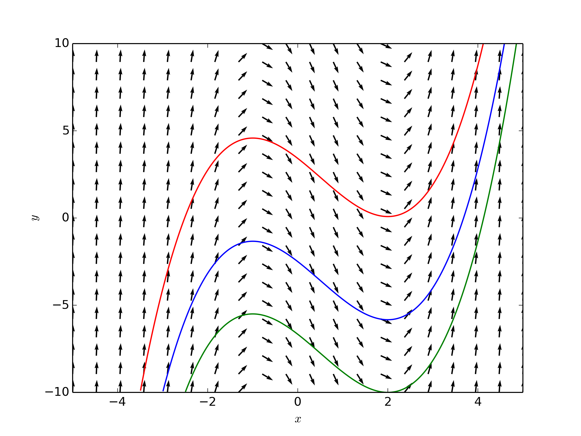
But what if the map we are trying to model cannot be described by a vector field, i.e. our data does not represent a continuous transformation? In the paper Augmented Neural ODEs out of Oxford, headed by Emilien Dupont, a few examples of intractable data for Neural ODEs are given. Let’s use one of their examples. Let A1 be a function such that A1(1)=−1 and A1(−1)=1.
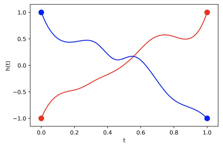
Above is a graph which shows the ideal mapping a Neural ODE would learn for A1, and below is a graph which shows the actual mapping it learns. Both graphs plot time on the x axis and the value of the hidden state on the y axis.
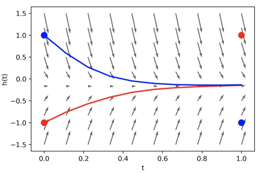
Hmmmm, what is going on here? The trajectories of the hidden states must overlap to reach the correct solution. However, with a Neural ODE this is impossible! ODE trajectories cannot cross each other because ODEs model vector fields. If the paths were to successfully cross, there would have to be two different vectors at one point to send the trajectories in opposing directions! The smooth transformation of the hidden state mandated by Neural ODEs limits the types of functions they can model. Since ResNets also roughly model vector fields, why can they achieve the correct solution for A1? Below is a graph of the ResNet solution (dotted lines), the underlying vector field arrows (grey arrows), and the trajectory of a continuous transformation (solid curves).
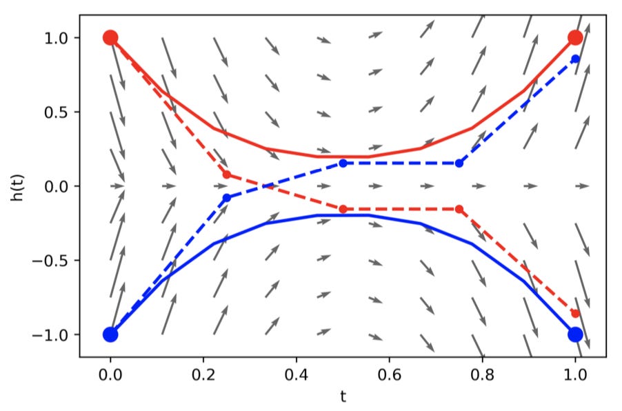
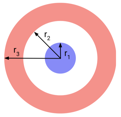
Because ResNets are not continuous transformations, they can jump around the vector field, allowing trajectories to cross each other. But with the continuous transformation, the trajectories cannot cross, as shown by the solid curves on the vector field. Thus Neural ODEs cannot model the simple 1-D function A1. In fact, any data that is not linearly separable within its own space breaks the architecture. For example, the annulus distribution below, which we will call A2
.
In this data distribution, everything radially between the origin and r1 is one class and everything radially between r2 and r3 is another class. The issue with this data is that the two classes are not linearly separable in 2D space. Since a Neural ODE is a continuous transformation which cannot lift data into a higher dimension, it will try to smush around the input data to a point where it is mostly separated. However, this brute force approach often leads to the network learning overly complicated transformations as we see below.
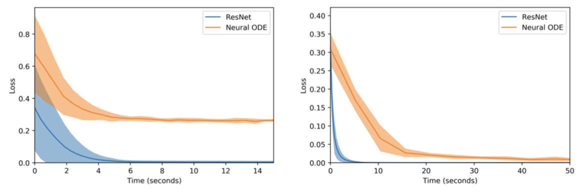
On the left, the plateauing error of the Neural ODE demonstrates its inability to learn the function A1, while the ResNet quickly converges to a near optimal solution. On the right, a similar situation is observed for A2. Peering more into the map learned for A2, below we see the complex squishification of data sampled from the annulus distribution.
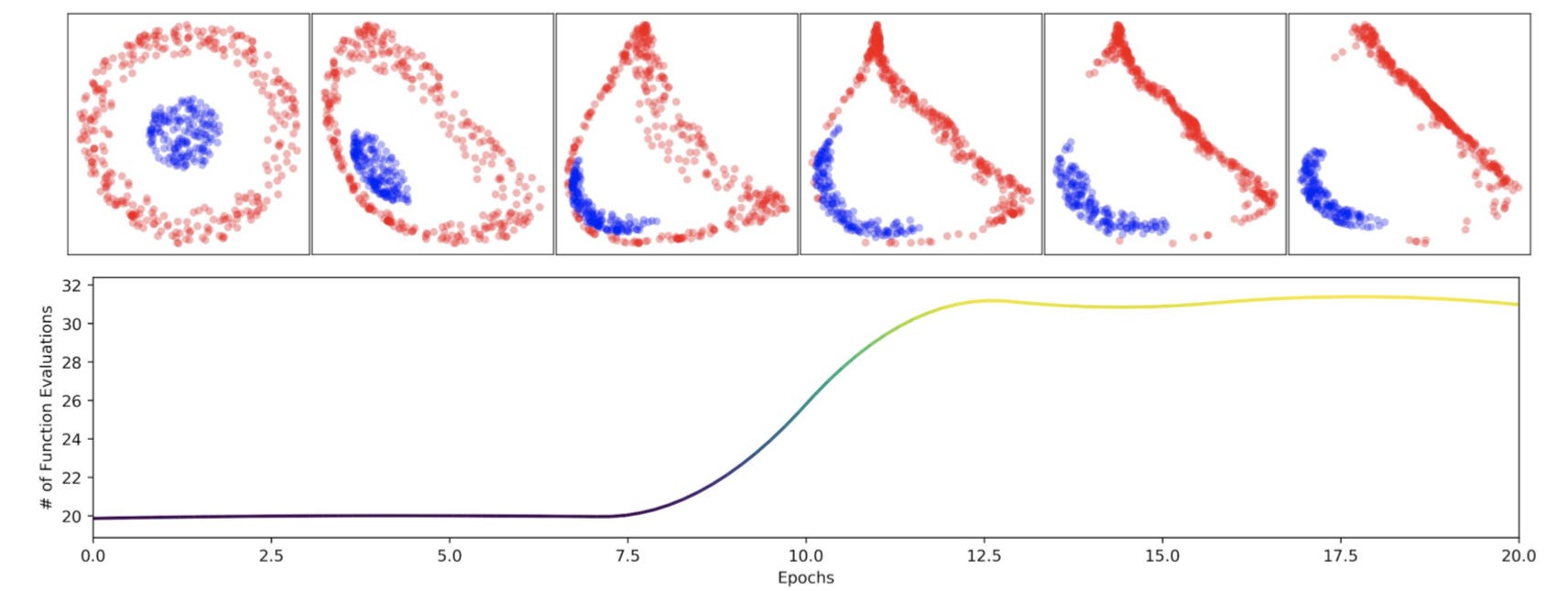
In the bottom plot of epochs vs ODESolve calls, we can observe that as the blue points are pushed through the red circle, the number of calls sharply increase. This inelegant mapping not only increases training and evaluation time, but also reduces generalizability as the decision boundary is artificially smushed and does not play to the symmetries of the distribution.
Fixing The Problem
The issue pinpointed in the last section is that Neural ODEs model continuous transformations by vector fields, making them unable to handle data that is not easily separated in the dimension of the hidden state. One solution is to increase the dimensionality of the data, a technique standard neural nets often employ. The way to encode this into the Neural ODE architecture is to increase the dimensionality of the space the ODE is solved in. If our hidden state is a vector in Rn, we can add on d extra dimensions and solve the ODE in Rn+d. The augmented ODE is shown below.
We are concatenating a vector of 0s to the end of each datapoint xxx, allowing the network to learn some nontrivial values for the extra dimensions. The data can hopefully be easily massaged into a linearly separable form with the extra freedom, and we can ignore the extra dimensions when using the network.
Below is a graphic comparing the number of calls to ODESolve for an Augmented Neural ODE in comparison to a Neural ODE for A2.
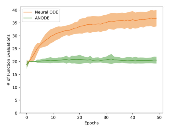
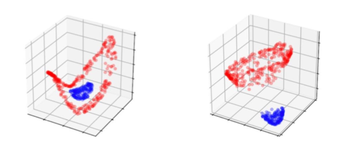
Instead of learning a complicated map in R2, the augmented Neural ODE learns a simple map in R3, shown by the near steady number of calls to ODESolve during training. The researchers also found in this experiment that validation error went to ~0 while error remained high for vanilla Neural ODEs. The graphic below shows A2 initialized randomly with a single extra dimension, and on the right is the basic transformation learned by the augmented Neural ODE.
One criticism of this tweak is that it introduces more parameters, which should in theory increase the ability of the model be default. However, the researchers experimented with a fixed number of parameters for both models, showing the benefits of ANODEs are from the freedom of higher dimensions. Another criticism is that adding dimensions reduces the interpretability and elegance of the Neural ODE architecture. The appeal of NeuralODEs stems from the smooth transformation of the hidden state within the confines of an experiment, like a physics model. In this case, extra dimensions may be unnecessary and may influence a model away from physical interpretability. Thus augmenting the hidden state is not always the best idea. Furthermore, the above examples from the A-Neural ODE paper are adversarial for an ODE based architecture. Practically, Neural ODEs are unnecessary for such problems and should be used for areas in which a smooth transformation increases interpretability and results, potentially areas like physics and irregular time series data.
Conclusions and Future Work
Neural ODEs present a new architecture with much potential for reducing parameter and memory costs, improving the processing of irregular time series data, and for improving physics models. The architecture relies on some cool mathematics to train and overall is a stunning contribution to the ML landscape.