
Towards Realistic Artificial Slow Motion

By Arjun Sripathy
If you’ve seen the Matrix you probably remember Neo dodging those bullets in the iconic scene shown above. But could you imagine that same scene without the slow motion? While probably still awesome, it would certainly lack the same appeal and impact. Until recently, quality slow motion has only been possible with high speed professional cameras. While this may be alright for moviemakers, it prevents people from fully capturing those special moments and amazing video opportunities that spontaneously present themselves in life. How likely are you to be carrying a professional camera in these situations? Fortunately, these may be limitations of the past—by the end of this post you will learn how any standard phone recording can artificially be transformed into a high quality, slow motion video!
More precisely, given a set of frames, we will discuss how to predict intermediate frames with the goal of artificially increasing the frame rate of the original video. This task is commonly known as frame interpolation. We will dive into different approaches one can take, starting with the basics and build towards a state-of-the-art method: Super SloMo.
Representing Videos
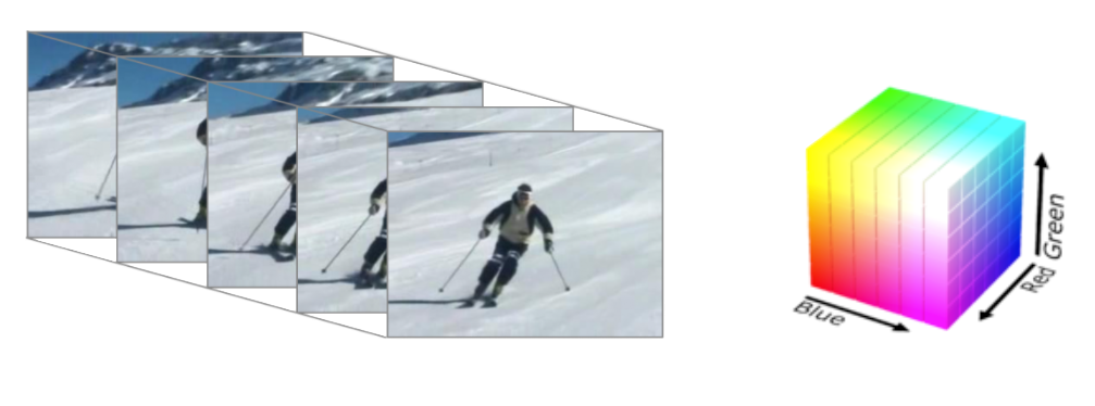
Let’s take a step back and consider how videos are represented in computers. Videos are internally represented by a series of images or video frames. The number of video frames that will be captured depends on the frame rate of the video. For the sake of perspective a standard cell phone video may have a frame rate of 30 frames per second: for every recorded second the video will have 30 frames. On the other hand, high speed recordings may have 240fps—or even higher! How to bridge this gap is the focus of this post, but first we have to address how images themselves are stored.
Computers are good with the numbers, so how may we effectively represent an image with them? The standard idea is to break up a picture into a grid of small chunks, or pixels, each of which has a constant color. The color of a pixel can be described by the combination of red, blue, and green components each of which typically range from 0 to 255. It turns out any color can be thought of as a combination of these three elementary components.
Below is a visual example. First we zoom into a small portion of the image to observe the presence of constant color pixels. Then we take a look at the R(ed)G(reen)B(lue) components of each pixel. Zooming back out we can represent the whole image as a matrix where each entry has the RGB values for the corresponding pixel.
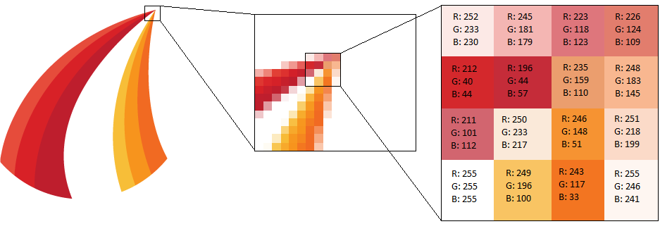
Pixel RGB values for a sub section of the corresponding image.
Putting it all together we can represent a video as a large matrix of the following dimensions (Note the 3 comes from the 3 components of RGB):
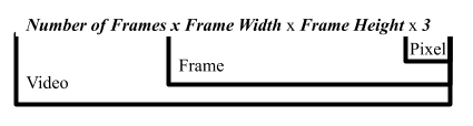
Dimensional breakdown for how videos are stored
Slower Playback
Now let us begin discussing our task of slowing down videos. One simple approach is to simply reduce the speed at which we play back the given frames. For example, if we playback a 30fps video at 15fps we are able to slow it down by a factor of 2. A video that was originally 1 minute long would now be stretched over 2 minutes. Cool so are we done?
Not quite! Simply stretching the timeline doesn’t increase the total number of frames in the video. The slowed video has a lower frame rate resulting in the stuttering effect shown below. (We will continue to reference the car example below throughout this post)
Original Speed
50% Playback Speed
25% Playback Speed
Reduced play back speed for car example
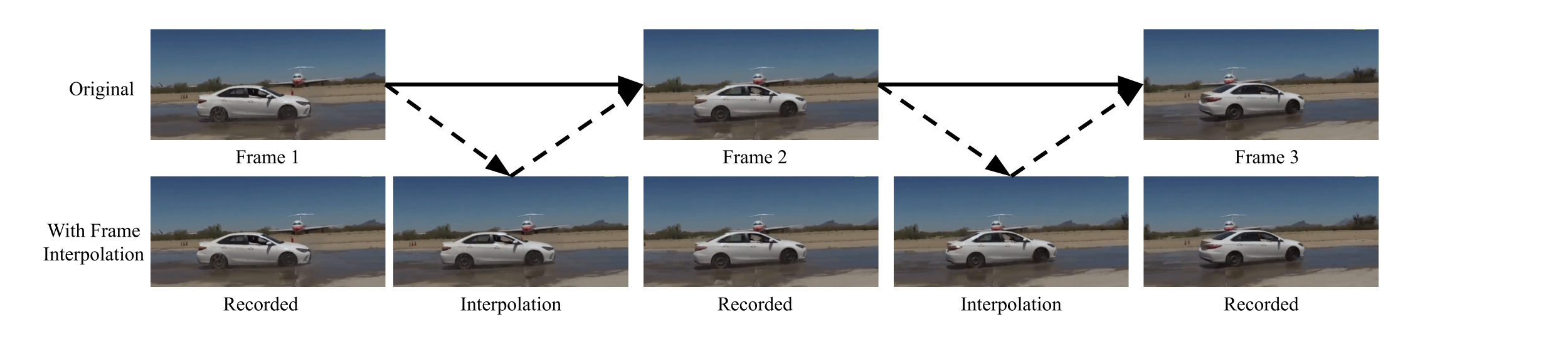
In order to make a slow-motion video that does not compromise the frame rate, we are going to need to increase the total number of frames in our video. Our approach will be to first reduce playback speed as we did here. Then we will interpolate between consecutive frames to smooth transitions and restore our original frame rate. For example, to achieve 25% speed we will introduce 3 interpolated frames between every pair of original ones (giving us 4 times as many frames as before). These interpolations will be our best guess for what a high speed camera would have captured in between the frames we have.

Demonstration of ideal frame interpolation on a car example
Linear Interpolation
Now we will discuss a naive approach to frame interpolation. Given two consecutive frames a natural way to predict an intermediate one is by taking the average of the two given. More precisely representing the frames as RGB matrices we may take the simple average between a pixel’s R, G, and B values in the two given frames to predict a frame that could reasonably occur between the two. For example, if the top left pixel in the first frame had RGB values (120,60,200) and in the second frame had RGB values (100,50,210) then in our interpolated frame the same pixel would have RGB values (110,55,205). This method is referred to as pixel-wise linear interpolation as we are smoothing the pixel-wise color differences between original frames.
When working with large images with little relative motion this method works well. More generally, when most of the pixels in consecutive frames are similar, this method will not have noticeable errors. However, the whole point of frame interpolation is to slow down dynamic videos; in this case, consecutive frames will be substantially different and pixel-wise interpolation will not work well. To demonstrate the issue with this method consider the following basic example.
Suppose we are recording a green ball in motion. We only have access to a 30fps camera, but we would like to convert our recording to 60fps, to slow it down by a factor of 2 maintaining the original quality. We’ll have to insert an interpolation between every pair of frames that our 30fps camera recorded.
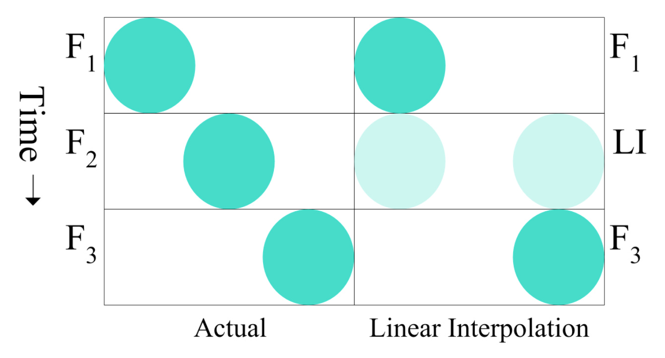
Demonstration of linear interpolation on a simple ball example
Here, we are zoomed in on a short time interval capturing the ball’s motion. The frames we would have got from a 60fps camera are on the left labeled F1, F2, and F3. However, we only got F1 and F3 for the same time interval.
We use pixel-wise linear interpolation between the two frames we have, to generate the frame labeled “LI” (Linear Interpolation) which aims to predict the missing frame, F2. Remember that in its most basic form linear interpolation does not actually locate objects and their motion, rather it simply averages pixels. The circle in F1 averages with the white space that occupies the same spot in F3, and similarly for the circle in F3 with the white space in F1. This results in two “half” circles where the circle starts and finishes, and no sign of the circle where it actually is at the target time. Since linear interpolation struggles in this simple circle-tracking scenario, it is no surprise that it also struggles with real-world video.
Consider the following example which demonstrates linear interpolation being used on the car example from before:
Linear Interpolation for a 50% slowdown on the running car example
The above attempts to slow down the original video by a factor of only 2, but immediately we observe the same issue that presented itself in the circle problem. Pixel-wise linear interpolation yields two “half cars”, one where the car was in the first frame and one for where it was in the second frame, instead of one car in the right spot. This problem is exacerbated due to the moving point of view. If we were to try to slow down the original video by a larger factor say 4, the result is even worse:
Linear Interpolation for a 25% slowdown on the running car example
The key issue with pixel-wise approaches is that they do not capture the motion of objects within the video. Thus, we need a model that takes into account how objects flow between frames…
Optical Flow
It turns out the key to better frame interpolation is the incorporation of optical flow. The term optical flow refers to the apparent motion of entities between two frames. It is important to understand that optical flow works at the pixel level, that is not at the object level. For every pixel in the frame we are interested in the “motion” of the color that previously occupied that space. This can be represented as a vector field that associates with each pixel position a velocity vector indicating the magnitude and direction of it’s color motion. Consider the example below:
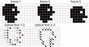
Optical flow vector field for simple black and white frames
The whole face moves between each of these frames, but only along the boundary do we observe a change in color. As a result only along this boundary do we have non zero optical flow. Further the arrows indicate the direction and magnitude of the corresponding motion.
A more realistic, complex example is shown below. Once again notice how optical flow vectors arise around boundaries of motion. Further notice how the optical flow vectors point opposite to the car’s direction. While the car is moving forward, everything visible in the frame is moving backwards.
Calculated optical flow for realworld car dashboard view
Traditional Optical Flow Computation
The method discussed below is not state-of-the-art but is important to learn about to properly understand the basis of optical flow computation. As is the case typically, optical flow is calculated between pairs of consecutive frames.
Traditionally we assume that an object won’t move by more than a few pixels between frames. For a target position, such a method would consider the neighboring locations in the second frame and locate where the original pixel’s color went. A more concrete example is as follows. Suppose originally a target position is bright red, but has different color in the second frame. We’d look in the vicinity of the target position and identify the closest pixel that is roughly bright red. Then we’d claim the optical flow for the target position as the displacement to that new bright red location. For example:
Target Position: (X,Y)=(10,25), First frame color: RGB (240,20,45) (Bright Red)
Second frame position (12,22) has RGB (235,23,38) (Roughly the same Bright Red). No point closer to (10,25) is of similar color.
⟹ Optical flow at (10,25) is (2,−3) (the displacement from (10,25) to (12,22))
If the pixel actually remains bright red in the second frame its corresponding vector would be (0,0)—indicating no local optical flow. Repeating this process for every position an optical flow vector field is determined that is both locally consistent as well as generally smooth to align with the underlying assumption of little relative motion between frames. Consistency means we do not have situations like multiple pixels claiming to have moved to the same place and smoothness refers to the idea that the optical flow vectors for nearby points should be similar.
The standard approach is to predict optical flow that minimizes the combination of these two components: the brightness constraint and the smoothness constraint.
First let’s discuss the brightness constraint in the context of the following example:
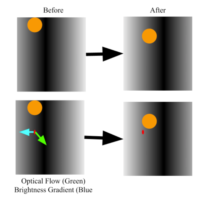
Optical flow and Brightness gradient for another simple ball example
The top two frames display two consecutive frames in a video. It appears that the pattern in this video moves down and to the right in the frame. The bottom two frames reflect the top ones, but with a specific position highlighted by a red dot. Shown in the bottom left frame are the optical flow at that point in green (down and to the right as expected) and the brightness gradient, which points towards the locally brighter areas, in blue (due left in this case).
Given that the pattern is locally moving against the brightness gradient, intuitively the original position will become brighter (take a moment to think about this) in the ensuing frame. As expected the position denoted by the red dot is brighter in the second frame than in the first. The brightness constraint is that the extent of the optical flow along the brightness gradient (the dot product between the two vectors), should roughly counter the observed change in brightness at the target position as seen in this example. In this sense, the optical flow should explain the change in brightness.
The second constraint is simpler, the smoothness constraint. It simply ensures that the optical flow is locally smooth. More precisely it encourages only small changes in optical flow for small changes in target position. These two constraints are optimized jointly, and the result is optical flow at each position of the given frame.
State-of-the-Art Optical Flow Computation
While the traditional principles remain important for understanding optical flow, more nuanced methods are used today for its computation. In order to function in cases of more significant motion between frames, recent approaches have leveraged deep learning to allow for greater flexibility in optical flow predictions. The method that is used by Super SloMo (which we’ll get to next!) is something known as a U-Net.
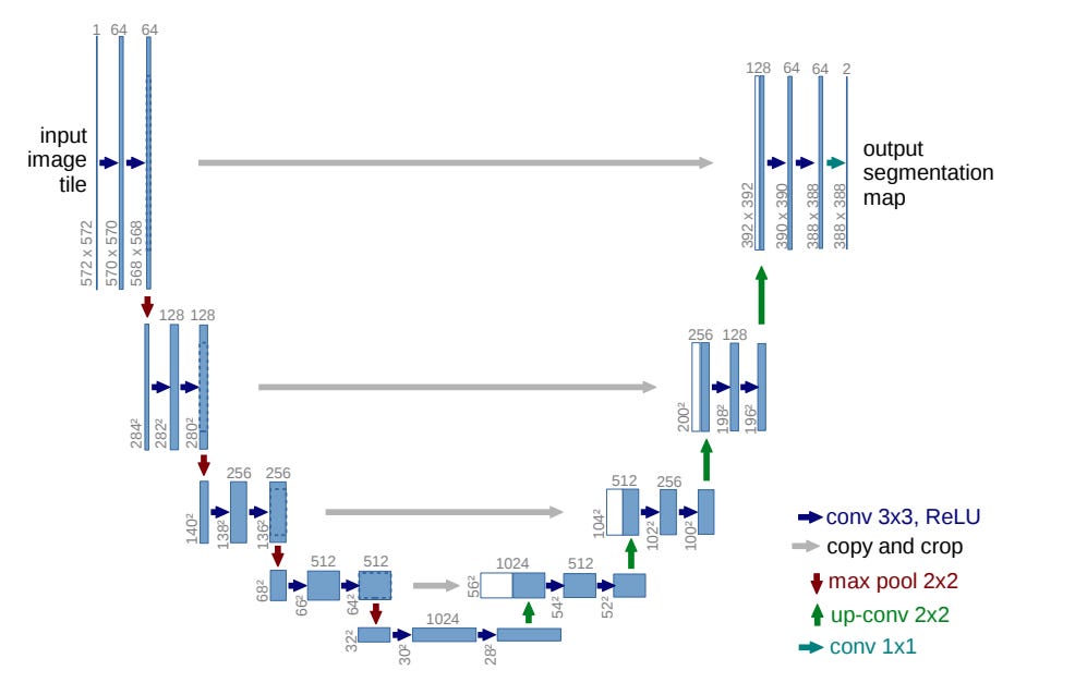
U-Net architecture visualization
The basic idea of U-Net is that you start with the two frames. Then you learn higher level, abstract features about the image that aren’t constrained to small local neighborhoods. Then you use these abstract features along with the original frames to precisely locate observed motion. By doing this we are able to surpass the limitations of earlier methods that were bound to a pixel’s small local neighborhood in computing its optical flow.
Super SloMo
Now we are finally ready to dive into Super SloMo. The model set out to make a number of key improvements to existing slow motion techniques. Among these improvements are the ability to predict more than one intermediate frame between two given ones without having error accumulation. In fact Super SloMo’s design allows for a variable number of intermediate frames. The other improvement is one that most researchers in the domain have been working towards: smoothly interpolating between frames that capture significant motion and/or occlusion (the concealment of objects within the frame).
At a high level their methodology can be broken down into three components: intermediate optical flow estimation, frame warping, and visibility weighting.
Intermediate Optical Flow Estimation
Super SloMo is based on using two frames F0 and F1, to predict Ft, where 0≤t≤1. They knew if they could accomplish this then variable number frame interpolation would be possible. Using the previously discussed U-Net architecture they are able to determine rough optical flows from F0 to F1 and vice versa, denoted by F0→1 and F1→0.
With these in place, we’d like to estimate the flow from the target time to either of the given frames. Mathematically we’d like to find optical flows Ft→1 and Ft→0 as they will help us transform the existing frames into the desired interpolation. There are two key ideas that help us here. The first being that motion is roughly linear between the two frames. Consider Ft→1. With our assumption of approximate linearity we have the following two estimates.
The multiplicative factor is because we only want flow for the last (1−t) time units. The latter estimation has a negative sign because F1→0 is moving in the opposite direction. The second key idea is that we should weigh the optical flow from the frame closer to time ttt more, since that one is likely to be more reliable. When t is closer to 0 we should weight F0→1 more. When t is closer to 1 we should weight F1→0 more. We can put all of this together in one equation as
And similarly
It turns out we can improve upon these linear approximations. To this end, Super SloMo uses an additional U-Net architecture simply for the purpose of fine tuning the optical flow for the target time t.
Frame Warping
In order to combine the optical flow with the given frames they define a backward warping function, g. It takes as input a frame and optical flow from the target time to the input frame. The idea is to combine these two pieces of information and estimate the frame at the target time. Super SloMo uses a simple linear interpolation method for this warping function, g. Meaning they move the pixels from the original frame in the manner prescribed by the optical flow to arrive at the target frame.
There are two ways we can get to the target frame. We can work forward from F0 or work backwards from F1. Instead of picking one option we do both and simply weigh each solution by how much we trust it. Once again we will trust the frame that is closer to our target time in a linear manner.
Visibility Weighting
Finally we have visibility weighting. In order to handle occlusion, or concealed objects, better we should trust the frame in which we can see the concealed object more. We quantify this notion with Vt←0 and Vt←1, where the former describes how visible the pixel was starting from frame 0 and the latter describes how visible it was after the target time until frame 1. We consider visibility as a relative quantity, so for any given pixel its value in Vt←0 and Vt←1 should sum to 1. If a pixel is more visible early on and gets concealed afterwards than its Vt←0 will be higher and vice versa.
Now we can finally formulate our result, that is our predicted target frame Ft based on what we have done so far.
such that
α0 represents how much we trust the forward approach starting from F0, and α0represents how much we trust the backward approach starting from F1. We normalize them so that they sum to 1 and our final predicted frame is a valid weighted output. In summary, we weight the first frame more when the target time is closer to 0 and/or the pixel is more visible in earlier times. Otherwise we weight the second frame more.
Evaluation
This model is optimized and evaluated with the aid of high definition videos. Certain frames of high speed recordings are concealed and the model is asked to recreate them using frame interpolation. The model is evaluated on it’s ability to predict frames with pixel values similar to the concealed ones. Additionally, there are metrics that capture how realistic and smooth the interpolated frames are. The bottom line is that there are many different, important metrics to consider and Super SloMo performs competitively in all of them. Here’s the car example from before slowed down using Super SloMo:
And just like that we have crisp, super slow motion videos generated from nothing more than standard cell phone recording! It’s only a matter of time before this technology becomes avaiable for broad usage by people around the world! If you are interested in reading more, below are some great places to start.
Super SloMo Nvidia News Page: https://news.developer.nvidia.com/transforming-standard-video-into-slow-motion-with-ai/
Super SloMo Paper: https://arxiv.org/pdf/1712.00080.pdf
Traditional Optical Flow Paper: http://image.diku.dk/imagecanon/material/HornSchunckOptical_Flow.pdf
U-Net Paper: https://arxiv.org/pdf/1505.04597.pdf